彩笔运维勇闯机器学习：多项式回归

前言

在之前的讨论中，讨论的都是线性回归，自变量与结果可以通过一条直线来解释。而今天讨论的问题，自变量与结果可能需要曲线来拟合，也就是所谓的 $x^n$，n>=2

开始探索

老规矩，先运行起来，再探索原理

1. scikit-learn

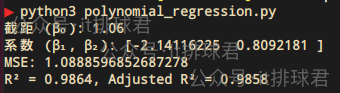
import numpy as np from sklearn.preprocessing import PolynomialFeatures from sklearn.linear_model import LinearRegression from sklearn.pipeline import Pipeline from sklearn.metrics import mean_squared_error, r2_score def adjusted_r2(r2, n, p): return 1 - (1 - r2) * (n - 1) / (n - p - 1) np.random.seed(0) x = np.linspace(-5, 5, 50) y_true = 0.8 * x**2 - 2 * x + 1 y_noise = np.random.normal(0, 1, len(x)) y = y_true + y_noise model_poly = Pipeline([ ('poly', PolynomialFeatures(degree=2)), ('linear', LinearRegression()) ]) model_poly.fit(x.reshape(-1, 1), y) y_pred = model_poly.predict(x.reshape(-1, 1)) r2 = r2_score(y, y_pred) n = len(x) p = 2 # 多项式阶数 r2_adj = adjusted_r2(r2, n, p) MSE = mean_squared_error(y, y_pred) coef = model_poly.named_steps['linear'].coef_ intercept = model_poly.named_steps['linear'].intercept_ print(f"截距 (β₀): {intercept:.2f}") print(f"系数 (β₁, β₂): {coef[1:]}") print("MSE:", MSE) print(f"R² = {r2:.4f}, Adjusted R² = {r2_adj:.4f}")

脚本！启动:

watermarked-polynomial_regression_1_1

2. 报告解读

又是熟悉的兄弟伙

MSE：均方误差，用于衡量模型预测值与真实值之间的差异，越趋于0越好
R²：决定系数，用于评估模型拟合优度的重要指标，其取值范围为[0, 1]
调整R²：调整决定系数，对R²的修正，惩罚不必要的特征（防止过拟合）。需要注意的是，这里计算调整决定系数的时候，p为多项式的阶数

在本次测试中，我们已经假定了多项式是： $$0.8x^2 - 2x + 1$$ 而最终模型为$$0.809x^2 - 2.141x + 1.06$$

深入理解多项式回归

1. 数学模型

\[\hat{y} = β_0 + β_1 x + β_2 x^2 + β_3 x^3 + \dots + β_n x^n \]

$β_0$ 叫做截距，在模型中起到了“基准值”的作用，就是当自变量为0的时候，因变量的基准值
$β_1$ $β_2$ $\dots$ $β_n$ 叫做自变量系数或者回归系数，描述了自变量对结果的影响方向和大小
- 多项式回归中，依然使用最小二乘法，是scikit-learn包的默认算法

2. 损失函数

线性回归通常使用均方误差（MSE）来作为损失函数，衡量测试值与真实值之间的差异

\[\text{MSE} = \frac{1}{n} \sum_{i=1}^{n} (y_i - \hat{y}_i)^2 \]

其中$y_i$是真实值，$\hat{y}_i$是预测值

正如前文提到，MSE中真实值与预测值，有平方计算，那就会放大误差，所以MSE可以非常有效的检测误差项

3. 决定系数

用于评估线性回归模型拟合优度的重要指标，其取值范围为 [0, 1]

\[R^2 = 1 - \frac{\sum_{i=1}^{n} (y_i - \hat{y}_i)^2}{\sum_{i=1}^{n} (y_i - \bar{y})^2} \]

其中$y_i$是真实值，$\hat{y}_i$是预测值，$\bar{y}$是均值

`scikit-learn`中的常用参数

这里有一个非常重要的参数，degree，这里表达了用几阶多项式来拟合模型。在本例中，使用的是2阶多项式，如果解释效果不好，可以尝试高阶多项式

如何选择回归模型

观察数据特征

最直观的方法，先将数据做散列点图，简单评估一下

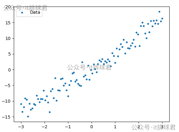
watermarked-polynomial_regression_1_2

一眼望去，可以用线性回归模型
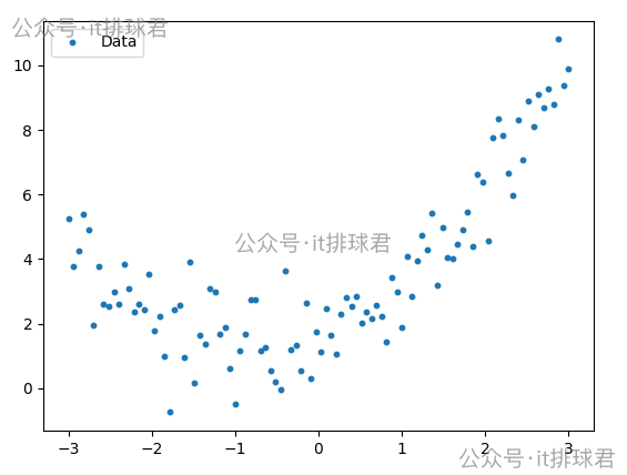
watermarked-polynomial_regression_1_3

这看起来是一条曲线，可以尝试用多项式模型

模型评估

先看线性模型与多项式模型的MSE与R²的对比

import numpy as np from sklearn.preprocessing import PolynomialFeatures from sklearn.linear_model import LinearRegression from sklearn.pipeline import Pipeline from sklearn.metrics import mean_squared_error, r2_score # 生成数据：y = 0.5x² + x + 噪声 np.random.seed(0) x = np.linspace(-3, 3, 100) y_true = 0.5 * x**2 + x y = y_true + np.random.normal(0, 1, len(x)) # 添加噪声 # 线性模型 model = LinearRegression() model.fit(x.reshape(-1, 1), y) y_pred = model.predict(x.reshape(-1, 1)) MSE = mean_squared_error(y, y_pred) r2 = r2_score(y, y_pred) print("线性模型：") print("R²:", r2) print("MSE:", MSE) print(f"截距 (β₀): {model.intercept_}") print(f"系数 (β): {model.coef_}\n") # 多项式模型 model2 = Pipeline([ ('poly', PolynomialFeatures(degree=2)), ('linear', LinearRegression()) ]) model2.fit(x.reshape(-1, 1), y) y_pred = model2.predict(x.reshape(-1, 1)) MSE = mean_squared_error(y, y_pred) r2 = r2_score(y, y_pred) print("多项式模型，阶数为2：") print("R²:", r2) print("MSE:", MSE) print(f"截距 (β₀): {model2.named_steps['linear'].intercept_}") print(f"系数 (β): {model2.named_steps['linear'].coef_[1:]}\n")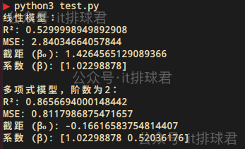

watermarked-polynomial_regression_1_4

明显是多项式模型解释性更好

残差图

所谓残差，是单个样本点的预测值与真实值之间的差

\[e_i=y_i - \hat{y}_i \]

$e_i$：残差
$y_i$：样本真实值
$\hat{y}_i$：样本预测值

import numpy as np import matplotlib.pyplot as plt from sklearn.preprocessing import PolynomialFeatures from sklearn.linear_model import LinearRegression from sklearn.pipeline import Pipeline from sklearn.metrics import mean_squared_error, r2_score # 生成数据：y = 0.5x² + x + 噪声 np.random.seed(0) x = np.linspace(-3, 3, 100) y_true = 0.5 * x**2 + x y = y_true + np.random.normal(0, 1, len(x)) # 添加噪声 def fit_poly(degree): model = Pipeline([ ('poly', PolynomialFeatures(degree=degree)), ('linear', LinearRegression()) ]) model.fit(x.reshape(-1, 1), y) y_pred = model.predict(x.reshape(-1, 1)) residuals = y - y_pred # 计算残差 return residuals degrees = [1, 2] plt.figure(figsize=(15, 4)) for i, degree in enumerate(degrees): residuals = fit_poly(degree) plt.subplot(1, 2, i+1) plt.scatter(x, residuals, s=10) plt.axhline(y=0, color='r', linestyle='--') plt.title(f"Residual Plots (degree={degree})") plt.xlabel("x") plt.ylabel("Residual") plt.show()

注意这里线性回归也可以直接通过指定degree=1来完成

脚本！启动

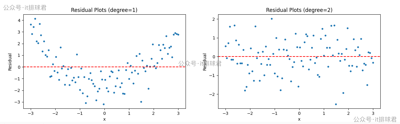
watermarked-polynomial_regression_1_5

左边是线性回归，右边是2次多项式回归
线性回归的残差呈现出明显的U型，说明未捕获非线性趋势
2次多项式的残差随机分散在0附近，无规律，说明拟合良好
正确的残差图不仅要体现出随机性，还要体现不可预测性

阶数选择

import numpy as np from sklearn.preprocessing import PolynomialFeatures from sklearn.linear_model import LinearRegression from sklearn.pipeline import Pipeline from sklearn.metrics import mean_squared_error, r2_score # 生成数据：y = 0.5x² + x + 噪声 np.random.seed(0) x = np.linspace(-3, 3, 100) y_true = 0.5 * x**2 + x y = y_true + np.random.normal(0, 1, len(x)) # 添加噪声 def adjusted_r2(r2, n, p): return 1 - (1 - r2) * (n - 1) / (n - p - 1) def fit_poly(degree): model = Pipeline([ ('poly', PolynomialFeatures(degree=degree)), ('linear', LinearRegression()) ]) model.fit(x.reshape(-1, 1), y) y_pred = model.predict(x.reshape(-1, 1)) MSE = mean_squared_error(y, y_pred) r2 = r2_score(y, y_pred) adj_r2 = adjusted_r2(r2, len(x), degree) print(f'阶数：{degree}，MSE：{MSE}，r2：{r2}, adj_r2：{adj_r2}') print('=='*10) degrees = [2, 3, 4, 5] for i, degree in enumerate(degrees): fit_poly(degree)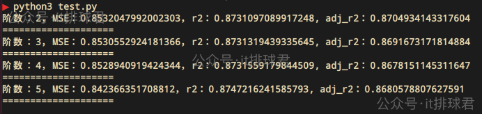

watermarked-polynomial_regression_1_6

通过2-5阶的遍历，发现2阶的调整决定系数是最高的
通过不断的升阶，虽然决定系数在慢慢上升，但是调整决定系数并没有上升，所以升阶并不能造成模型有实质的改变。这个问题在线性回归详细描述过
2阶多项式就是拟合度更高的模型

对比：

原始的函数为 $y=0.5x^{2}+x$ ，通过截距与回归系数，计算出不同阶的方程，然后与原函数对比

import numpy as np from sklearn.preprocessing import PolynomialFeatures from sklearn.linear_model import LinearRegression from sklearn.pipeline import Pipeline # 生成数据：y = 0.5x² + x + 噪声 np.random.seed(0) x = np.linspace(-3, 3, 100) y_true = 0.5 * x**2 + x y = y_true + np.random.normal(0, 1, len(x)) # 添加噪声 def adjusted_r2(r2, n, p): return 1 - (1 - r2) * (n - 1) / (n - p - 1) def format(args): n = len(args) terms = [] for i, coeff in enumerate(args): power = n - 1 - i if coeff == 0: continue term = "" if coeff > 0 and terms: term += "+" elif coeff < 0: term += "-" coeff = abs(coeff) if coeff != 1 or power == 0: term += str(round(coeff, 3)) if power > 0: term += "*" if power > 0: term += "x" if power > 1: term += f"^{power}" terms.append(term) return "".join(terms) if terms else "0" def fit_poly(degree): model = Pipeline([ ('poly', PolynomialFeatures(degree=degree)), ('linear', LinearRegression()) ]) model.fit(x.reshape(-1, 1), y) coef = model.named_steps['linear'].coef_ intercept = model.named_steps['linear'].intercept_ args = coef[1:].tolist() args.append(intercept) s = format(args) print(f'多项式{degree}阶：{s}') print('=='*10) degrees = [2, 3, 4, 5] for i, degree in enumerate(degrees): fit_poly(degree)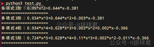

watermarked-polynomial_regression_1_7

进行对比，可以通过该网站画出函数图

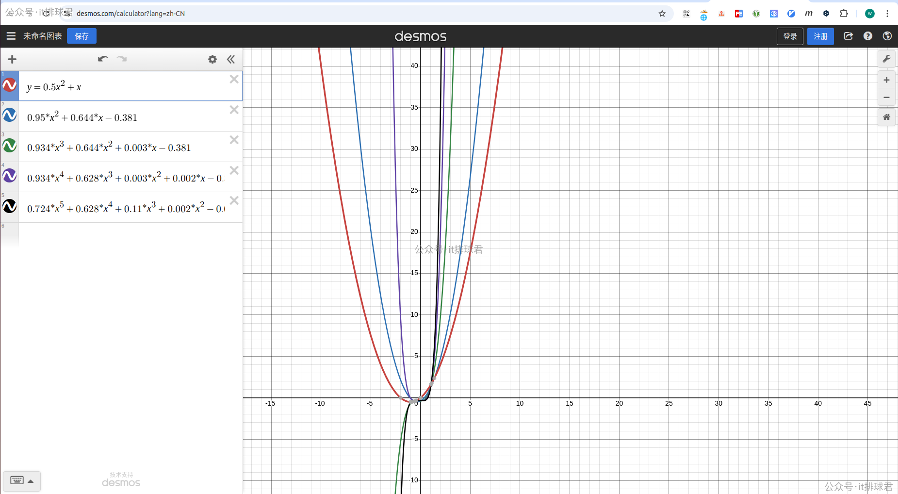
watermarked-polynomial_regression_1_8

红色是原二次函数，而蓝色是经过噪声之后拟合的二次函数，与红色是最接近的，越往Y轴靠，阶数越高

pipeline

它可以将多个数据处理步骤和机器学习模型组合成一个整体的工作流

之前在lasso回归那里，在lasso回归之前，需要将数据标准化，再进行模型训练

scaler = StandardScaler() X_scaled = scaler.fit_transform(X2) lasso = Lasso(alpha=0.1) lasso.fit(X_scaled, y2)

通过pipleline，可以直接写成一个工作流

from sklearn.pipeline import Pipeline lasso_pipe = Pipeline([ ('scaler', StandardScaler()), ('lasso', Lasso(alpha=0.1)) ]) lasso_pipe.fit(X2, y2)

当然还有本次多项式回归中提到的

model_poly = Pipeline([ ('poly', PolynomialFeatures(degree=2)), ('linear', LinearRegression()) ])

可以看到，先进行PolynomialFeatures，这就是所谓的升阶操作，再进行LinearRegression线性回归。在sklearn中，多项式的处理方式本质就是先升阶，再进行线性回归，所以线性回归的理论都可以用在多项式回归当中

联系我

联系我，做深入的交流

至此，本文结束
在下才疏学浅，有撒汤漏水的，请各位不吝赐教...

本文来自博客园，作者：it排球君，转载请注明原文链接：https://www.cnblogs.com/MrVolleyball/p/19056400

本文版权归作者和博客园共有，欢迎转载，但未经作者同意必须在文章页面给出原文连接，否则保留追究法律责任的权利。